This week we are delving deeper into R and using ggplot. For me, the interesting importance of ggplot, is its relationship to the Grammar of Graphics by Leland Wilkins, published in 1999. I once found the study of Linguistics fascinating and always felt that mathematics was a type of language and I feel partner dancing such as ballroom and latin is a type of language as well, a language whose grammar changes subtly with each new partner. And now I learn that similar to the grammar of language, good graphics consist of defined elements that assist us in creating/determining the meaning of the graph. In ggplot the primary three elements are the Data, Aesthetics and Geometries. The Data is the dataset to be described, the Aesthetics are the look of the graphic, the scale the data is mapped to and the Geometries relate to the visual elements used. I copied and pasted some of the commands in the Module 11 presentation and was happy to get the same results.


Being contrary, I wanted to try to do something with an alternate dataset rather than just make some chanegs in the above displays. Unfortunately, I didn’t have much luck so I turned to Data Camp for some tutorials. Data Camp has free tutorials on many topics and only requires you to sign up. I was impressed with the quality of the tutorials. They are designed well with simple instructions and small video presentations explaining specifics in more detail. The introduction to ggplot starts with basically copying and pasting commands to see how they are executed and to understand how you can go wrong just like the assignment instructions!
In experimenting with the commands, the str() is very useful. the Data Camp tutorial is turning to the ‘Diamonds’ data set and str(diamonds) gives us:
str(diamonds)
Classes ‘tbl_df’, ‘tbl’ and ‘data.frame’: 53940 obs. of 10 variables:
$ carat : num 0.23 0.21 0.23 0.29 0.31 0.24 0.24 0.26 0.22 0.23 …
$ cut : Ord.factor w/ 5 levels “Fair”<“Good”<..: 5 4 2 4 2 3 3 3 1 3 …
$ color : Ord.factor w/ 7 levels “D”<“E”<“F”<“G”<..: 2 2 2 6 7 7 6 5 2 5 …
$ clarity: Ord.factor w/ 8 levels “I1″<“SI2″<“SI1″<..: 2 3 5 4 2 6 7 3 4 5 …
$ depth : num 61.5 59.8 56.9 62.4 63.3 62.8 62.3 61.9 65.1 59.4 …
$ table : num 55 61 65 58 58 57 57 55 61 61 …
$ price : int 326 326 327 334 335 336 336 337 337 338 …
$ x : num 3.95 3.89 4.05 4.2 4.34 3.94 3.95 4.07 3.87 4 …
$ y : num 3.98 3.84 4.07 4.23 4.35 3.96 3.98 4.11 3.78 4.05 …
$ z : num 2.43 2.31 2.31 2.63 2.75 2.48 2.47 2.53 2.49 2.39 …
 This allows us to use the appropriate command types for the different variable types, as you can see this function tells us if a variable is numerical or ordinal, etc. The instructions ask us to copy the command to create a scatter plot and to add a line. We are then asked to use some other commands.
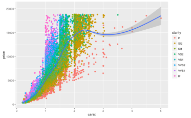
This command: ggplot(diamonds, aes(x = carat, y = price))+geom_point(aes(col=clarity)) +geom_smooth(), produced this graphic:
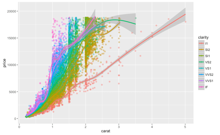
 This command: ggplot(diamonds, aes(x = carat, y = price)) +geom_point()+ geom_smooth(aes(col=clarity)), produced this.
Neither is correct for this exercise though and the instructions continue with a new term ‘alpha’ set to 0.04 and to not include the geom_smooth. When I ran this command: ggplot(diamonds, aes(x = carat, y = price))+geom_point(aes(col=clarity, alpha=0.04)) I got a graph similar to the colored points above but with transparency based on clarity, but this was still not correct. The correct command was: ggplot(diamonds, aes(x = carat, y = price, col = clarity)) +geom_point(alpha = 0.4). I decided to end with everything thrown in: ggplot(diamonds, aes(x = carat, y = price, col = clarity))+geom_point(alpha = 0.4)+geom_smooth(aes(col=clarity)). I would change the labels if I cared enough about the clarity of diamonds and its relationship to their value but since I am radically opposed to the diamond trade, I will leave it as is and play with changing text in my next project.


Leave a comment